Introduction to Tree Data Structure for Beginners

A tree is a data structure used in computer science to represent hierarchical relationships between objects.

It consists of nodes (or elements) connected by edges, which define the relationships between them.

Each node can have zero, one, or multiple child nodes, and the connections between the nodes are referred to as branches.

Trees are useful in various applications, such as representing hierarchical data, organizing data for quick search, insertions, and deletions, and as a foundation for many advanced data structures like binary search trees, heaps, and trie.

One common type of tree is a binary tree, in which each node has at most two children, usually referred to as the left and right child.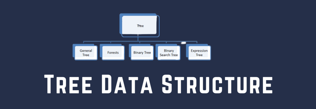

This structure is particularly useful for organizing data in a way that allows for efficient searching and sorting operations.

Terminologies

Here are the main components of a tree data structure:

1. Root: The root is the top-most node in the tree, and it has no parent. There is only one root node in a tree.
2. Parent node: A parent node is a node that has at least one child. In other words, it is a node that branches to other nodes in the tree.
3. Child node: A child node is a node that has a parent. It is connected to its parent by an edge.
4. Leaf node: A leaf node is a node with no children. It is at the bottom level of the tree.
5. Sibling nodes: Nodes that share the same parent are called siblings.
6. Level: The level of a node is the number of edges in the path from the root to the node. The root has a level of 0, its children have a level of 1, and so on.
7. Height: The height of a tree is the maximum number of edges in the longest path from the root to a leaf node. The height of an empty tree is -1.

Root

The root is the top-most node of a tree data structure and serves as the starting point for the entire tree. It is the only node in the tree that does not have a parent. All other nodes in the tree can be reached by following a unique path of edges from the root.

Let’s consider a simple example of a tree representing the management hierarchy of a company:

      CEO (Root)
      /      \
   VP1        VP2
  /  \        /  \
M1   M2     M3   M4

In this example, the tree consists of the following nodes:

• Root: CEO (Chief Executive Officer)
• Level 1: VP1 (Vice President 1) and VP2 (Vice President 2)
• Level 2: M1, M2, M3, and M4 (Managers)

Here, the CEO is the root node because it is at the top of the hierarchy and has no parent. It is also the starting point for the management hierarchy. From the root node, you can traverse down the tree through the branches to reach every other node, which represents the different levels of management in the company.

The root node plays a crucial role in tree-based algorithms, as it is the starting point for any traversal, search, or modification operations.

Parent node

A parent node in a tree data structure is a node that has one or more child nodes connected to it.

In other words, a parent node is a node that branches out to other nodes in the tree.

Each child node has exactly one parent, while a parent node can have multiple children.

Let’s revisit the example of the company’s management hierarchy:

      CEO (Root)
      /      \
   VP1        VP2
  /  \        /  \
M1   M2     M3   M4

In this tree:

1. The CEO node is the root and the parent of nodes VP1 and VP2.
2. VP1 is a parent node with child nodes M1 and M2.
3. VP2 is a parent node with child nodes M3 and M4.

Parent nodes are essential in representing the hierarchical relationships between nodes in the tree.

They provide structure and help define the connections between different levels in the hierarchy.

In tree-based algorithms, parent nodes play a vital role in operations such as traversals, searches, insertions, and deletions.

For example, when searching for a specific node or value, you often start from the root and navigate through parent nodes until you reach the desired node or value.

Similarly, when inserting a new node, you first find the appropriate parent node to connect it to, and so on.

Child node

A child node in a tree data structure is a node that has a parent node. In other words, a child node is a node that is connected to another node, called its parent, through an edge or branch.

Each child node has exactly one parent, but a parent node can have multiple children.

Let’s use the company’s management hierarchy:

       CEO (Root)
       /      \
    VP1        VP2
   /  \        /  \
 M1   M2     M3   M4

In this management hierarchy tree:

1. VP1 and VP2 are child nodes of the CEO.
2. M1 and M2 are child nodes of VP1.
3. M3 and M4 are child nodes of VP2.

Child nodes in this example represent the hierarchical relationships between different levels of management within the company.

They help structure the connections between various management roles and provide a means to navigate the hierarchy.

In the context of this example, if you wanted to find the direct subordinates of VP1, you would look at its child nodes, M1 and M2. Similarly, to find the direct subordinates of VP2, you would look at its child nodes, M3 and M4.

The management hierarchy example demonstrates how child nodes play an essential role in representing hierarchical relationships and connecting different levels in a tree data structure.

In algorithms that involve tree traversal, searching, inserting, or deleting nodes, child nodes are crucial.

For example, if you want to search for a specific node or value in the tree, you start from the root node and navigate through child nodes until you find the desired node or value. Similarly, when deleting a node, you may need to adjust its child nodes to maintain the tree’s structure.

Leaf node

A leaf node, also known as a terminal node, is a node in a tree data structure that does not have any child nodes. It is located at the bottom level of the tree, and it represents the end of a branch.

Let’s use the management hierarchy example to illustrate leaf nodes:

     CEO (Root)
     /      \
   VP1        VP2
  /  \        /  \
M1   M2     M3   M4

In this management hierarchy tree:

1. M1, M2, M3, and M4 are leaf nodes.

Leaf nodes represent the endpoints of branches in the tree and often correspond to the final or most specific elements in a hierarchy.

In the context of the management hierarchy example, leaf nodes represent the lowest level of management, where there are no further subordinates. These managers (M1, M2, M3, and M4) do not have any direct reports, and they are at the end of the management chain.

Leaf nodes play an essential role in tree-based algorithms, as they often signify the termination point for various operations such as traversals, searches, or insertions.

For example, during a depth-first search traversal, when you reach a leaf node, you know that you have explored all nodes along that branch and can backtrack to explore other branches in the tree.

Sibling node

Sibling nodes are nodes in a tree data structure that share the same parent node. In other words, sibling nodes are nodes that are located on the same level of the tree and connected to the same parent through branches.

Let’s use the management hierarchy example to illustrate sibling nodes:

     CEO (Root)
     /      \
   VP1        VP2
  /  \        /  \
M1   M2     M3   M4

In this management hierarchy tree:

1. VP1 and VP2 are sibling nodes, as they share the same parent node, CEO.
2. M1 and M2 are sibling nodes, as they share the same parent node, VP1.
3. M3 and M4 are sibling nodes, as they share the same parent node, VP2.

Sibling nodes represent elements in the tree that have a similar relationship with their parent and are on the same level of the hierarchy. They help in understanding the structure and organization of the tree and provide a means to navigate between related nodes within the same level.

In the context of the management hierarchy example, sibling nodes can represent peers or colleagues within the same management level. For example, M1 and M2 are both managers reporting to VP1, making them siblings in the hierarchy.

Sibling nodes play an essential role in tree-based algorithms, particularly during traversals. For instance, during a breadth-first search traversal, you visit all sibling nodes at a given level before moving on to the next level.

Level

In a tree data structure, the level of a node refers to the number of edges or branches in the path from the root node to the node itself. The root node has a level of 0, its children have a level of 1, their children have a level of 2, and so on.

The level indicates the depth of a node in the tree and helps in understanding the hierarchical relationships between nodes in the tree.

Let’s use the management hierarchy example to illustrate tree levels:

      CEO (Root)
     /      \
   VP1        VP2
  /  \        /  \
M1   M2     M3   M4

In this management hierarchy tree, the nodes are located at the following levels:

1. Level 0: CEO (Root node)
2. Level 1: VP1 and VP2 (Child nodes of the CEO)
3. Level 2: M1, M2, M3, and M4 (Child nodes of VP1 and VP2)

The levels in this example represent the different tiers of management within the company. As you go deeper into the tree, you move further down the management hierarchy.

Tree levels play a crucial role in tree-based algorithms, particularly during traversals. For example, in a breadth-first search (BFS) traversal, you visit all nodes at a given level before moving on to the next level.

Similarly, the level of a node is important for algorithms that balance or optimize tree structures, such as in AVL trees or B-trees.

Height

The height of a tree is the maximum number of edges (branches) in the longest path from the root node to a leaf node (the furthest node from the root). In other words, the height indicates the depth of the tree, which represents the maximum number of levels in the tree. The height of an empty tree is -1.

Let’s use the management hierarchy example to illustrate tree height:

      CEO (Root)
     /      \
   VP1        VP2
  /  \        /  \
M1   M2     M3   M4

In this management hierarchy tree, we can determine the height as follows:

1. Start at the root node (CEO).
2. Count the number of edges in the longest path to a leaf node (M1, M2, M3, or M4).
3. In this case, there is one edge from the CEO to VP1 or VP2, and another edge from VP1 or VP2 to M1, M2, M3, or M4. The longest path consists of 2 edges.

So, the height of this tree is 2.

The height of a tree is an important factor in determining the efficiency of tree-based algorithms, such as searching, inserting, or deleting nodes.

In general, the lower the tree’s height, the faster these operations can be performed. Balanced trees, like AVL trees or Red-Black trees, aim to minimize the height to optimize search and modification operations.

Properties

Trees have several key properties that define their structure and behavior. Here are some of the most important properties of trees:

These properties help define the structure, organization, and behavior of trees, making them a versatile and efficient data structure for various applications, such as representing hierarchical relationships, organizing data, and optimizing search and modification operations.

It expands the versatility and applicability of trees in various domains, such as computer science, mathematics, and data organization.

Trees can be tailored to meet the needs of specific algorithms or applications by adjusting their structure, branching, or traversal methods, making them a powerful and adaptable data structure.

1. Hierarchical structure: A tree data structure represents a hierarchical relationship between its elements, with each element (except the root) having exactly one parent and zero or more children.
2. Root node: A tree has a unique starting point called the root node, which does not have a parent. All other nodes in the tree can be reached by following a unique path of edges from the root.
3. Parent-child relationship: In a tree, each node has a parent-child relationship with its connected nodes. A parent node has one or more child nodes, while a child node has exactly one parent.
4. Sibling nodes: Nodes that share the same parent are called sibling nodes. They represent elements with a similar relationship to their parent and are on the same level of the tree.
5. Leaf nodes: A leaf node, also known as a terminal node, is a node that does not have any child nodes. Leaf nodes represent the endpoints of branches in the tree.
6. Level: The level of a node is the number of edges in the path from the root node to that node. The root node has a level of 0, its children have a level of 1, their children have a level of 2, and so on.
7. Height: The height of a tree is the maximum number of edges in the longest path from the root node to a leaf node. The height of an empty tree is -1.
8. Ordered or unordered: Trees can be ordered or unordered. In an ordered tree, the children of a node are ordered in a specific way, such as in a binary search tree. In an unordered tree, there is no specific order for the child nodes.
9. Balanced or unbalanced: A tree can be balanced or unbalanced. Balanced trees, like AVL trees or Red-Black trees, ensure that the height of the tree is minimized, which optimizes search and modification operations. An unbalanced tree may have a height that is significantly larger, resulting in less efficient operations.
10. Degree: The degree of a node is the number of its child nodes. The degree of a tree is the maximum degree of all its nodes. The degree determines the branching factor of a tree, which can affect the tree’s height and the efficiency of certain operations.
11. Forest: A forest is a collection of disjoint trees, meaning there is no connection between any nodes across different trees in the forest. Forests can be used to represent multiple separate hierarchical structures or sets of data.
12. Binary tree: A binary tree is a tree in which each node has at most two child nodes, usually distinguished as left and right children. Binary trees are commonly used for organizing data in a sorted or hierarchical manner, like in binary search trees and heaps.
13. Multiway tree: A multiway tree is a tree that allows each node to have more than two children, such as a ternary tree (three children per node) or an M-ary tree (M children per node). Multiway trees can be useful for efficiently organizing large datasets, like in B-trees or trie data structures.
14. Path and traversal: The path in a tree refers to the sequence of nodes and edges connecting two nodes in the tree. Traversal is the process of visiting all the nodes in a tree in a specific order. There are several tree traversal methods, including pre-order, in-order, post-order, and level-order (breadth-first search).

Types of Trees

There are several types of trees in computer science, each with its own characteristics and use cases. Here are some common types of trees:

1. Binary Tree: A binary tree is a tree in which each node has at most two child nodes, usually referred to as the left child and the right child. Binary trees are often used as the basis for more specialized tree structures.
2. Binary Search Tree (BST): A binary search tree is a binary tree with the property that the value of each node is greater than or equal to all values in its left subtree and less than or equal to all values in its right subtree. BSTs are used for efficient searching, insertion, and deletion operations.
3. Balanced Binary Search Trees: These are binary search trees that automatically maintain a balanced state to ensure that operations are performed efficiently. Some examples include:
   • AVL Tree: A self-balancing binary search tree that maintains a balance factor of -1, 0, or 1 for every node.
   • Red-Black Tree: A self-balancing binary search tree that uses color attributes (red or black) to maintain a balanced structure.
4. Heap: A heap is a specialized binary tree that satisfies the heap property, in which the key of each node is either greater than or equal to (max-heap) or less than or equal to (min-heap) its children’s keys. Heaps are commonly used to implement priority queues.
5. Trie (Prefix Tree): A trie is a tree-like data structure used to store a dynamic set of strings or associative arrays. Tries allow efficient searching, insertion, and deletion operations for string-based keys.
6. B-Tree: A B-Tree is a self-balancing tree data structure that maintains a sorted order and allows for efficient searching, insertion, and deletion operations. B-Trees have a variable number of child nodes and are commonly used in databases and file systems.
7. M-ary Tree: An M-ary tree is a tree in which each node has at most M children. An M-ary tree is a generalization of the binary tree and can be used to represent more complex hierarchical relationships.
8. K-D Tree (k-dimensional tree): A k-d tree is a binary search tree used for organizing points in k-dimensional space. K-D trees enable efficient range and nearest-neighbor searches in multidimensional datasets.
9. Suffix Tree: A suffix tree is a compressed trie containing all the suffixes of a given text as keys and their positions in the text as values. Suffix trees are used for pattern matching and string processing algorithms.
10. R-Tree: An R-Tree is a tree data structure used for storing spatial data, such as rectangles or polygons. R-Trees enable efficient querying and manipulation of spatial data.
11. N-ary Tree (General Tree): An N-ary tree is a tree in which each node can have any number of child nodes. N-ary trees can be used to represent complex hierarchical relationships or multiway branching structures.

These trees are designed to optimize specific operations, such as searching, insertion, deletion, or data organization, based on the nature of the data and the requirements of the application.

Operations

There are several fundamental operations that can be performed on tree data structures. Some of the most common operations include insertion, deletion, searching, and traversal. In this article, we will focus on binary search trees (BST) as an example, and provide pseudocode and explanations for each operation:

Node Insertion in BST:

To insert a new node into a binary search tree, we start at the root and traverse the tree until we find an appropriate position for the new node, which maintains the BST property.

Pseudocode for insertion:

function insert(node, value):
    if node is None:
        return create_new_node(value)
    if value < node.value:
        node.left = insert(node.left, value)
    else:
        node.right = insert(node.right, value)
    return node

We start at the root node and compare the value we want to insert with the current node’s value. If the value is smaller, we move to the left child; otherwise, we move to the right child. We continue this process recursively until we reach an empty position where we can insert the new node.

Node Deletion in BST:

To delete a node in a binary search tree, we need to consider three cases: the node has no children, the node has one child, or the node has two children.

Pseudocode for deletion:

function delete(node, value):
    if node is None:
        return None
    if value < node.value:
        node.left = delete(node.left, value)
    elif value > node.value:
        node.right = delete(node.right, value)
    else:
        if node.left is None:
            return node.right
        elif node.right is None:
            return node.left
        else:
            node.value = find_min(node.right)
            node.right = delete(node.right, node.value)
    return node

function find_min(node):
    while node.left is not None:
        node = node.left
    return node.value

If the node to delete has no children, we simply remove it. If the node has one child, we remove the node and replace it with its child. If the node has two children, we find the minimum value in the right subtree, replace the node’s value with this minimum value, and delete the minimum value node from the right subtree.

Node Searching in BST:

To search for a value in a binary search tree, we start at the root and traverse the tree following the same logic as in the insertion process.

Pseudocode for searching:

function search(node, value):
    if node is None or node.value == value:
        return node
    if value < node.value:
        return search(node.left, value)
    else:
        return search(node.right, value)

We start at the root node and compare the value we want to search for with the current node’s value. If the value is smaller, we move to the left child; otherwise, we move to the right child. We continue this process recursively until we find the value or reach an empty position, indicating that the value is not in the tree.

Tree Traversal in BST:

Traversal is the process of visiting all the nodes in a tree in a specific order. There are several traversal methods, including in-order, pre-order, post-order, and level-order (breadth-first search).

Pseudocode for in-order traversal:

function in_order_traversal(node):
    if node is not None:
        in_order_traversal(node.left)
        print(node.value)
        in_order_traversal(node.right)

In an in-order traversal, we visit the left subtree, process the current node, and then visit the right subtree. This traversal method returns the nodes in a

sorted order for a binary search tree, making it particularly useful for extracting ordered data from the tree.

Pseudocode for pre-order traversal:

function pre_order_traversal(node):
    if node is not None:
        print(node.value)
        pre_order_traversal(node.left)
        pre_order_traversal(node.right)

In a pre-order traversal, we process the current node, visit the left subtree, and then visit the right subtree. Pre-order traversal is often used for copying a tree or generating a prefix expression of the tree.

Pseudocode for post-order traversal:

function post_order_traversal(node):
    if node is not None:
        post_order_traversal(node.left)
        post_order_traversal(node.right)
        print(node.value)

In a post-order traversal, we visit the left subtree, visit the right subtree, and then process the current node. Post-order traversal is useful for deleting nodes in the tree or generating a postfix expression of the tree.

Pseudocode for level-order traversal (breadth-first search):

function level_order_traversal(root):
    if root is None:
        return

    queue = create_empty_queue()
    enqueue(queue, root)

    while not is_empty(queue):
        node = dequeue(queue)
        print(node.value)

        if node.left is not None:
            enqueue(queue, node.left)

        if node.right is not None:
            enqueue(queue, node.right)

In a level-order traversal, also known as a breadth-first search, we visit all nodes at the same level before moving on to the next level. We use a queue to keep track of nodes to visit. Level-order traversal is useful for applications like searching for the shortest path in a tree or determining the level of nodes.

Find Minimum in BST:

Find the node with the smallest value in the BST. Start from the root node and follow the left child pointers until you reach a node with no left child.

Pseudocode for Minimum:

function find_min(node):
    if node is None:
        return None
    while node.left is not None:
        node = node.left
    return node

Find Maximum in BST:

Find the node with the largest value in the BST. Start from the root node and follow the right child pointers until you reach a node with no right child.

Pseudocode for Maximum:

function find_max(node):
    if node is None:
        return None
    while node.right is not None:
        node = node.right
    return node

Find Predecessor in BST:

Given a node, find the node with the largest value that is smaller than the given node’s value. If the node has a left child, the predecessor is the maximum node in the left subtree. Otherwise, search up the tree from the node to the root, and the first right ancestor is the predecessor.

Pseudocode for Predecessor:

function find_predecessor(node):
    if node is None:
        return None

    if node.left is not None:
        return find_max(node.left)

    ancestor = node.parent
    while ancestor is not None and node == ancestor.left:
        node = ancestor
        ancestor = ancestor.parent

    return ancestor

Find Successor in BST:

Given a node, find the node with the smallest value that is larger than the given node’s value. If the node has a right child, the successor is the minimum node in the right subtree. Otherwise, search up the tree from the node to the root, and the first left ancestor is the successor.

Pseudocode for Successor:

function find_successor(node):
    if node is None:
        return None

    if node.right is not None:
        return find_min(node.right)

    ancestor = node.parent
    while ancestor is not None and node == ancestor.right:
        node = ancestor
        ancestor = ancestor.parent

    return ancestor

Find the Height of BST:

Calculate the height of the BST, which is the maximum number of edges in the longest path from the root node to a leaf node.

Pseudocode for Height:

function find_height(node):
    if node is None:
        return -1

    left_height = find_height(node.left)
    right_height = find_height(node.right)

    return max(left_height, right_height) + 1

Find the Size of the BST:

Calculate the total number of nodes in the BST.

Pseudocode for Size:

function get_size(node):
    if node is None:
        return 0
    return 1 + get_size(node.left) + get_size(node.right)

Check if Tree is BST:

Determine if a given binary tree is a binary search tree or not by checking if it satisfies the BST property.

Pseudocode for Check if BST:

function is_bst(node, min_value=-inf, max_value=inf):
    if node is None:
        return True

    if node.value < min_value or node.value > max_value:
        return False

    left_check = is_bst(node.left, min_value, node.value)
    right_check = is_bst(node.right, node.value, max_value)

    return left_check and right_check

Balancing an AVL Tree:

Rebalance the BST to ensure that the height is minimized, which can optimize search, insertion, and deletion operations. This operation is performed on self-balancing binary search trees, such as AVL trees or Red-Black trees.

Here, I’ll provide an example of AVL tree balancing, which relies on the balance factor of each node (the difference between the heights of the left and right subtrees).

function insert(node, value):
    if node is None:
        return create_new_node(value)

    if value < node.value:
        node.left = insert(node.left, value)
    else:
        node.right = insert(node.right, value)

    node.height = 1 + max(find_height(node.left), find_height(node.right))

    balance_factor = get_balance_factor(node)

    # Left-Left case
    if balance_factor > 1 and value < node.left.value:
        return rotate_right(node)

    # Right-Right case
    if balance_factor < -1 and value > node.right.value:
        return rotate_left(node)

    # Left-Right case
    if balance_factor > 1 and value > node.left.value:
        node.left = rotate_left(node.left)
        return rotate_right(node)

    # Right-Left case
    if balance_factor < -1 and value < node.right.value:
        node.right = rotate_right(node.right)
        return rotate_left(node)

    return node

function get_balance_factor(node):
    if node is None:
        return 0
    return find_height(node.left) - find_height(node.right)

function rotate_right(y):
    x = y.left
    t2 = x.right

    x.right = y
    y.left = t2

    y.height = 1 + max(find_height(y.left), find_height(y.right))
    x.height = 1 + max(find_height(x.left), find_height(x.right))

    return x

function rotate_left(x):
    y = x.right
    t2 = y.left

    y.left = x
    x.right = t2

    x.height = 1 + max(find_height(x.left), find_height(x.right))
    y.height = 1 + max(find_height(y.left), find_height(y.right))

    return y

This pseudocode demonstrates how AVL tree balancing works. When inserting a new node, we first perform a regular BST insertion.

Then, we update the height of the current node and calculate the balance factor. If the balance factor is greater than 1 or less than -1, the tree is unbalanced, and we need to perform rotations to balance the tree.

There are four possible cases: Left-Left, Right-Right, Left-Right, and Right-Left. For each case, we perform one or two rotations to balance the tree.

Application

Tree data structures are used in various real-life applications due to their hierarchical nature, flexibility, and efficiency. Here are some examples where tree data structures are employed:

1. File System: The hierarchical structure of folders and files in a computer’s file system can be represented as a tree, with each folder as an internal node and each file as a leaf node. The tree’s root represents the top-level directory.
2. XML and HTML Parsing: XML and HTML documents have a tree-like structure, with tags being nodes and attributes being properties of the nodes. Trees are used to represent, parse, and manipulate the structure of these documents.
3. Game Trees: In artificial intelligence, game trees are used to represent possible moves and outcomes in two-player games like chess or tic-tac-toe. Each node in the tree represents a game state, and its children represent the resulting game states after each possible move.
4. Decision Trees: In machine learning, decision trees are used for classification and regression tasks. Each internal node represents a decision based on an attribute, and each leaf node represents the outcome or class label. Decision trees are a popular choice for their interpretability and ease of implementation.
5. Syntax Trees: In compilers and programming language parsers, syntax trees represent the syntactic structure of the source code. Each node in the tree represents a grammar rule, and the tree structure reflects the nesting of language constructs.
6. Organization Charts: In business and management, organization charts represent the hierarchy of roles within an organization. The tree’s root represents the top executive, and each node represents a position within the organization, with its children being subordinates.
7. Trie (Prefix Tree): Tries are used in applications like autocomplete, spell checkers, and IP routing. They store a dynamic set of strings, allowing efficient search, insertion, and deletion operations. Each node in the trie represents a character, and the edges connect characters that form a prefix.
8. Binary Search Trees (BST): BSTs are used for efficient searching, insertion, and deletion operations. They are the underlying data structure for various ordered data structures, such as sets, maps, and priority queues. Examples of BSTs include AVL trees, Red-Black trees, and B-trees.
9. Huffman Coding Trees: Huffman coding is a lossless data compression algorithm that assigns variable-length codes to input characters based on their frequencies. The algorithm builds a binary tree, with each leaf node representing a character and its associated binary code.
10. Abstract Syntax Trees (AST): ASTs are used in compilers and interpreters to represent the abstract syntactic structure of the source code. They are derived from the syntax tree and omit certain language-specific details, making them suitable for semantic analysis and code generation.

Pros and Cons of Tree Data Structure

Each data structure has its own advantages and disadvantages depending on the specific use case. Here, I’ll compare the pros and cons of tree data structures to those of hash-based structures, lists, and arrays:

Pros:

1. Hierarchical Structure: Trees can naturally represent hierarchical relationships, making them suitable for various applications like file systems, organization charts, and XML parsing.
2. Ordered: Trees, especially Binary Search Trees, can maintain elements in a sorted order, making it efficient for searching, insertion, and deletion operations.
3. Logarithmic Time Complexity: Balanced trees like AVL trees and Red-Black trees have O(log n) time complexity for search, insertion, and deletion operations.
4. Versatility: Trees have many variations (BST, Trie, B-tree, etc.) that are optimized for specific tasks, making them suitable for a wide range of applications.
5. Range Queries: Trees, especially Binary Search Trees, allow for efficient range queries (e.g., finding all elements between two values), which can be difficult or inefficient with other data structures like arrays or hash-based structures.
6. Prefix Matching: Certain tree structures, like Tries, are specifically designed for efficient prefix matching operations, making them ideal for tasks such as autocompletion, spell checking, and IP routing.
7. Adaptive Performance: Some tree structures, like Splay Trees, adapt their shape based on access patterns, which can lead to improved performance for specific use cases, such as when certain elements are accessed more frequently than others.
8. Multi-Dimensional Data: Trees can be extended to handle multi-dimensional data efficiently. Examples include k-d trees and R-trees, which are used for tasks like spatial indexing, nearest neighbor search, and range search in multiple dimensions.
9. Persistent Data Structure: Trees can be used to implement persistent data structures, which retain previous versions of the data structure even after modifications. This can be useful for tasks like version control systems, undo/redo functionality, and database management.
10. Concurrency Control: Tree data structures like Concurrent Skip Lists, AVL trees, and B-trees have been adapted for concurrent access and modification, which can be useful in multi-threaded and distributed systems.
11. Memory Management: Trees can be useful for memory management tasks, such as in the implementation of memory allocators or garbage collectors. For example, Buddy Memory Allocation uses a binary tree structure to manage memory blocks.
12. Extensibility: Trees are highly extensible and can be customized to suit specific needs. For example, Augmented Trees store additional information at each node, which can be used to optimize certain operations, like finding the order statistics, maintaining interval overlaps, or supporting other domain-specific functionality.

Cons:

1. Space Overhead: Trees have higher space overhead due to the storage of pointers/references for child nodes.
2. Complexity: Trees can be more complex to implement and maintain compared to arrays, lists, or hash-based structures.
3. Rebalancing: Some tree structures, like AVL trees and Red-Black trees, require rebalancing after insertion or deletion operations to maintain their efficiency. This can increase the complexity of the implementation and the time spent on these operations.
4. Traversal: Unlike arrays and lists, trees do not have a natural linear order for traversal, which can make it more challenging to iterate through all elements. While there are tree traversal techniques (e.g., in-order, pre-order, post-order), they are generally more complicated to implement than a simple loop.
5. Dependency on Height: The efficiency of many tree operations depends on the height of the tree. An unbalanced tree can have a height of O(n) in the worst case, leading to poor performance. Balancing the tree can help mitigate this issue, but it also adds complexity to the implementation.
6. Search Inefficiency for Unsorted Data: Trees are most efficient when they are used to represent ordered data. When dealing with unsorted data, trees are less efficient for searching compared to hash-based structures, which offer average-case O(1) search time.
7. Pointer Chasing: Accessing tree nodes often involves following multiple pointers, which can lead to poor cache locality and increased cache misses. This can have a negative impact on the overall performance of tree operations, especially on large data sets.
8. Increased Implementation Effort: Compared to simpler data structures like arrays and lists, trees often require more effort to implement correctly. This can be a disadvantage when trying to quickly develop a solution or when working with a team that is less familiar with tree data structures.
9. Difficulty in Parallelization: Due to the hierarchical nature of trees and the dependencies between nodes, it can be challenging to parallelize tree operations effectively. Other data structures, like arrays or hash-based structures, may offer better opportunities for parallelization and improved performance on multi-core systems.